Advanced options
Overview
The topics in this document are:
Data management 2
We can do a lot of calculations and data manipulations with R. First of all, we can use R as a calculator:
2 + 4## [1] 6We can save the result as an object in R. Then it is displayed in the upper right pane. With <- we assign an object
x <- 2 + 4
x
## [1] 6
Vectors
Vectors are a series of different values. With c() we can combine elements into a vector. Let’s say I want to make a vector “v” with 4 values; 1,2,3,4.
v <- c(1,2,3,4)
v
## [1] 1 2 3 4class(v)## [1] "numeric"Since the elements of “v” are numbers, the class is numeric. I can also make a vector of text elements. In that case, the class of the vector will be “character”.
v2 <- c("Monday", "Tuesday", "Wednesday", "Friday")
v2
## [1] "Monday" "Tuesday" "Wednesday" "Friday"class(v2)## [1] "character"The function c() can also be used to combine two vectors.
v3 <- c(v,v2)
v3
## [1] "1" "2" "3" "4" "Monday" "Tuesday"
## [7] "Wednesday" "Friday"class(v3)## [1] "character"Notice how all the elements of v3 are now strings.
Matrices and data frames
A matrix is a two dimensional vector. We can make a matrix with the function matrix().
m1 <- matrix(c(1:9), nrow = 3)
m1
## [,1] [,2] [,3]
## [1,] 1 4 7
## [2,] 2 5 8
## [3,] 3 6 9class(m1)## [1] "matrix" "array"The matrix m1 is filled with the number 1 through 9 (with c(1:9) I make a sequence of numbers). The matrix is filled in vertically. By specifying nrow = 3 R knows how many rows I want. Now compare this with the following matrix:
m2 <- matrix(c(1:9), nrow = 3, byrow = TRUE)
m2
## [,1] [,2] [,3]
## [1,] 1 2 3
## [2,] 4 5 6
## [3,] 7 8 9Can you guess what byrow = TRUE does?
For our data sets, we often use the class data.frame. I can make my matrix into a data frame:
data2 <- as.data.frame(m2)
data2
## V1 V2 V3
## 1 1 2 3
## 2 4 5 6
## 3 7 8 9class(data2)## [1] "data.frame"You can also build your data set by combining vectors using the cbind() function:
data3 <- as.data.frame(cbind(v, v2))
data3
## v v2
## 1 1 Monday
## 2 2 Tuesday
## 3 3 Wednesday
## 4 4 FridayNote Notice the difference between data3 and the vector v3 we created earlier.
Certain row numbers or colum numbers can be accessed using the square brackets [,]. A number before the comma gives this row number. This code gives me the first row:
mtcars[1,] ## mpg cyl disp hp drat wt qsec vs am gear carb
## Mazda RX4 21 6 160 110 3.9 2.62 16.46 0 1 4 4
A number after the comma shows this column number (or variable number). Here we show the second column:
mtcars[,2] ## [1] 6 6 4 6 8 6 8 4 4 6 6 8 8 8 8 8 8 4 4 4 4 8 8 8 8 4 4 4 8 6 8 4
Transform data from wide to long format
For analyses of data sets with repeated measurements the data need to be in the so-called “long” format instead of the “wide” format. Data are in wide format if each patient has one row and the repeated measurements are different variables. Data are in the long format if there is one variable for the repeated measurement, and a patient has multiple rows.
The following dataset data_wide is in the wide format.
head(data_wide)## id group M_1 M_2 M_3 M_4
## 1 1 1 27.5 20.1 26.9 20.8
## 2 2 1 19.1 20.9 22.7 19.1
## 3 3 1 24.4 19.1 22.6 25.3
## 4 4 1 24.0 13.3 26.6 15.5
## 5 5 1 21.6 19.5 20.0 20.7
## 6 6 2 13.0 29.7 20.9 28.5It has 10 patients and 6 variables. The variables M_1, M_2, M_3, M_4 are a continuous marker, measured at 4 time points.
Using the library data.table and the function melt() we can transform the wide data into long. The melt function has a few important options: id are the variables that are not time-varying, such as a baseline covariate. measure is the variable that is time-varying. There can be multiple repeated measurements. Using the function patterns(), all variables including M will be included as the repeated measure, so I do not need to type c(M_1, M_2, M_3, M_4). With value.name the repeated variable is given a new name and variable.name tells us which measurement it is.
library(data.table)
data_long <- melt(setDT(data_wide), id = c('id', 'group'),
                  measure = patterns("M"),
                  value.name = c('M'), variable.name = "Time")

levels(data_long$Time) <-  c(1, 2, 3, 4)

data_long <- data_long[order(data_long$id),]
head(data_long)
## id group Time M
## 1: 1 1 1 27.5
## 2: 1 1 2 20.1
## 3: 1 1 3 26.9
## 4: 1 1 4 20.8
## 5: 2 1 1 19.1
## 6: 2 1 2 20.9
dplyr
Cheatsheet for the dplyr package from the tidyverse:
https://nyu-cdsc.github.io/learningr/assets/data-transformation.pdf
Advanced graphs
Coming soon!
Survival analysis
A comprehensive guide to survival analysis in R can be found here: Survival Analysis in R Companion - By Dimitris Rizopoulos
Mixed effects models
Mixed models in general
One of the assumptions of (linear) regression models is that the observations are independent of each other. This assumptions does not hold in situations of clustered or hierarchical data.
In multicenter studies, patients are clustered within centers of the study. In longitudinal studies with repeated measurements per patient, observations from one patient are clustered in that patient. This can influence the analyses of a study, because observations within a cluster might be more correlated than observation between different clusters.
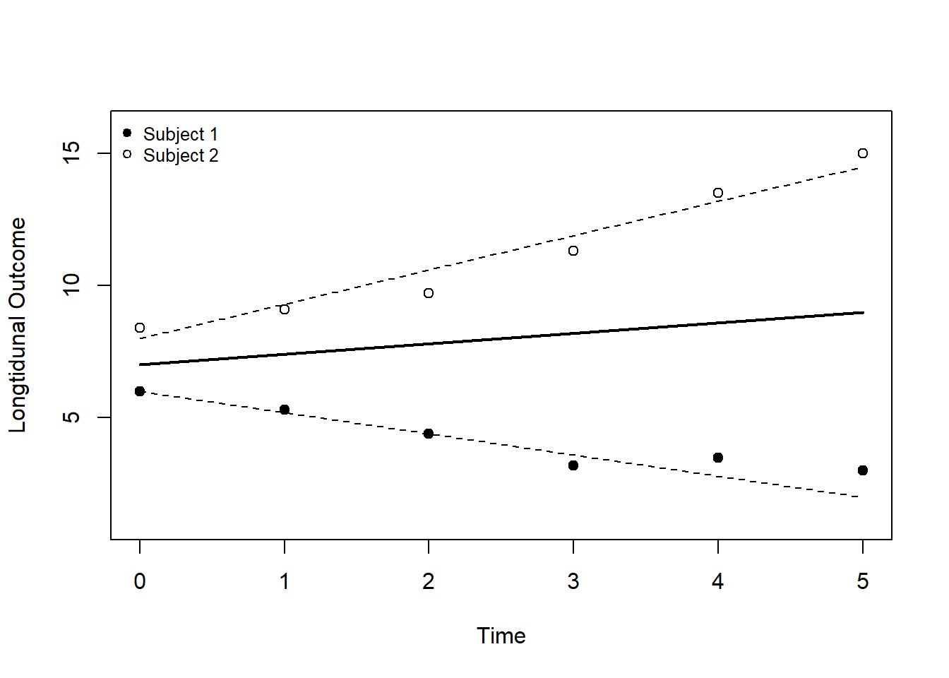
One framework possible for clustered is the mixed effects model. This is regression model that combines fixed (or population) effects with random (or subject-specific) effects.
The graph below visualizes a mixed effects model for repeated measures on two patients (Subject 1 and Subject 2). The thick black line is the population effect estimated by the fixed effects. Through the random effects, every patient has a specific intercept and slope indicated by the dashed lines.
Install the package(s)
Two libraries are used most often for mixed effects models in R; nlme and lme4. Here I will use lme4for the analyses, however a data set available in nlme is used as an example.
install.packages(lme4)
install.packages(nlme)
library(lme4)
library(nlme)The lme4 package does not provide p-values for the models. Some explanation on why by the author of the package, can be found here. The package lmerTest will provide you with p-values, however caution is needed in interpreting them!
The dataset for the example is Orthodont
data(Orthodont)
head(Orthodont)
## Grouped Data: distance ~ age | Subject
## distance age Subject Sex
## 1 26.0 8 M01 Male
## 2 25.0 10 M01 Male
## 3 29.0 12 M01 Male
## 4 31.0 14 M01 Male
## 5 21.5 8 M02 Male
## 6 22.5 10 M02 Maledim(Orthodont)## [1] 108 4The dataset consists of 108 observations, from 27 different subjects. The below code, calculates the number of unique values for each variable.
sapply(Orthodont, function(x) length(unique(x)))## distance age Subject Sex
## 27 4 27 2We can also see that there are 4 ages at which the distances are measured and two sexes.
Visualize longitudinal data
A good way to visualize longitudinal data is with a spaghetti plot. Measurements from the same subject are connected with a line.
library(ggplot2)
p <- ggplot(data = Orthodont) +
  geom_point(aes(x = age, y = distance, group = Subject, colour = Sex)) +
  geom_line(aes(x = age, y = distance, group = Subject, colour = Sex)) +
  theme_classic()
p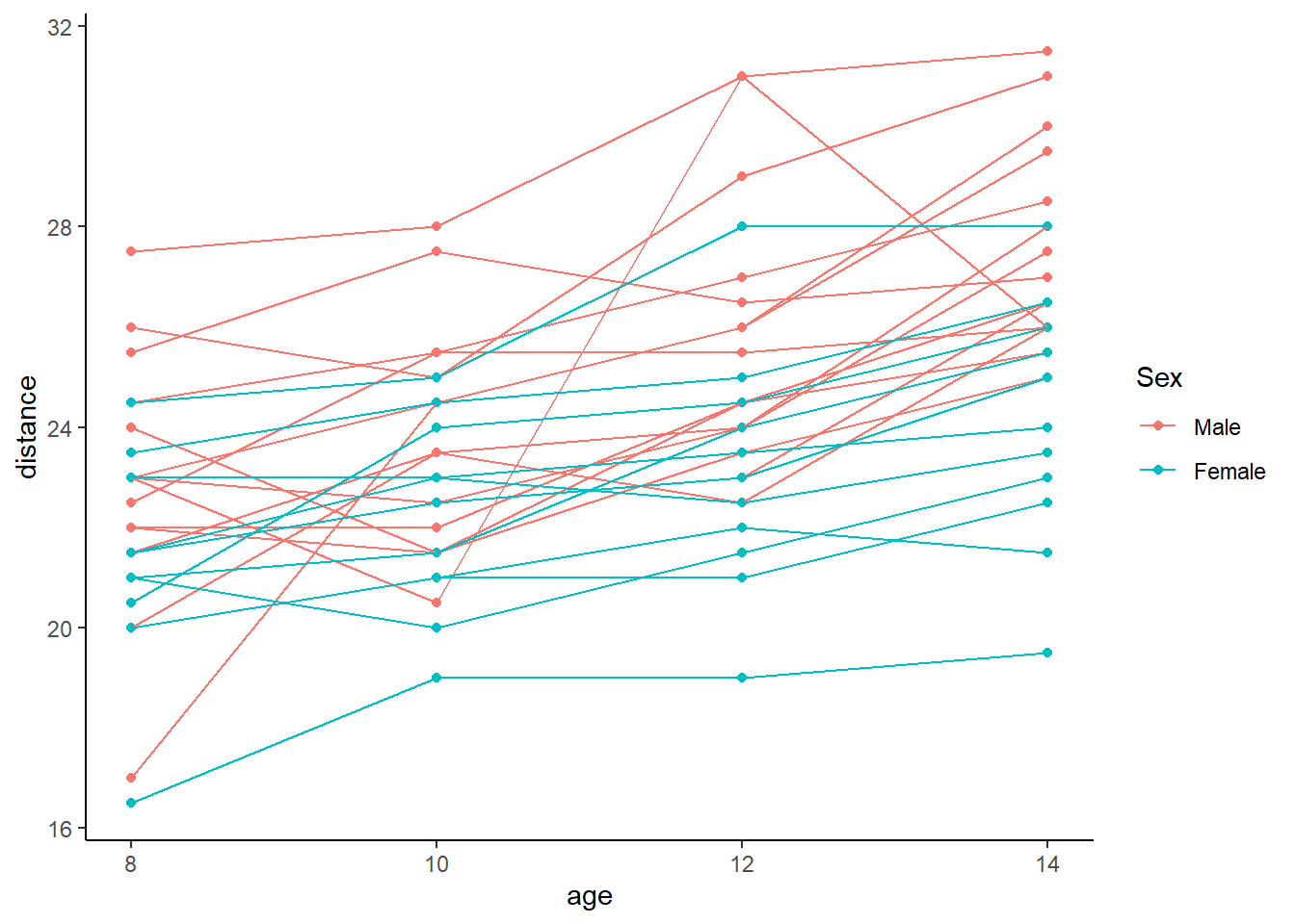
Based on the plot, overall the subjects seem to increase as age increases and Males seem to have a higher distance than Females.
Fit the model
We fit the mixed effects model, for which the code is similar to a linear regression model. In the fixed effect, we include age, sex and an interaction. In model fm1 we estimate random intercepts with the code (1 | Subject), allowing every subject their own intercept.
fm1 <- lmer(distance ~ age*Sex + (1 | Subject), data = Orthodont) With the summary command the results of the model can be obtained.
summary(fm1)## Linear mixed model fit by REML ['lmerMod']
## Formula: distance ~ age * Sex + (1 | Subject)
## Data: Orthodont
##
## REML criterion at convergence: 433.8
##
## Scaled residuals:
## Min 1Q Median 3Q Max
## -3.5980 -0.4546 0.0158 0.5024 3.6862
##
## Random effects:
## Groups Name Variance Std.Dev.
## Subject (Intercept) 3.299 1.816
## Residual 1.922 1.386
## Number of obs: 108, groups: Subject, 27
##
## Fixed effects:
## Estimate Std. Error t value
## (Intercept) 16.3406 0.9813 16.652
## age 0.7844 0.0775 10.121
## SexFemale 1.0321 1.5374 0.671
## age:SexFemale -0.3048 0.1214 -2.511
##
## Correlation of Fixed Effects:
## (Intr) age SexFml
## age -0.869
## SexFemale -0.638 0.555
## age:SexFeml 0.555 -0.638 -0.869The output provides us with both the random effects, which are estimators of the variance of each random effect (+possible covariances between random effects), and the fixed effects. The fixed effects are the population estimators and can be interpreted similar to the output of a linear regression model.
Compare two models
In model fm2 we additionally include random slopes with (age | Subject).
fm2 <- lmer(distance ~ age*Sex + (age | Subject), data = Orthodont) With the `anova() function we can compare the models to see which model provides a better fit of the data
anova(fm1, fm2)## Data: Orthodont
## Models:
## fm1: distance ~ age * Sex + (1 | Subject)
## fm2: distance ~ age * Sex + (age | Subject)
## npar AIC BIC logLik deviance Chisq Df Pr(>Chisq)
## fm1 6 440.64 456.73 -214.32 428.64
## fm2 8 443.81 465.26 -213.90 427.81 0.8331 2 0.6593From the AIC measure (smaller is better) we conclude that the random intercepts model provides a better fit of the data.
Evaluate the residuals
An important assumption of the mixed model is the normality of the residuals. They can be evaluated with the following code:
model <- fm1

par(mfrow = c(2,2))

# Are the residuals random noise?
residuals <- resid(model)
plot(fitted(model), residuals)
abline(0,0)

# Is the response variable a reasonable linear function
# of the fitted values?
plot(fitted(model), Orthodont$distance)

# Are the residuals normally distributed?
qqnorm(residuals)
qqline(residuals)
hist(residuals)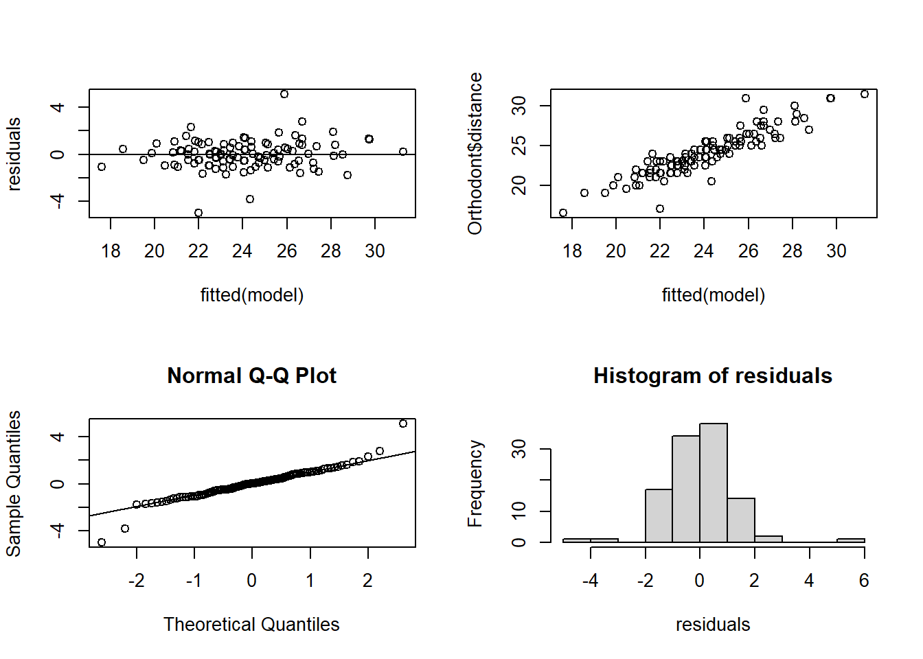
There is a slight deviation from normality in the tails of the residuals, but not too much.
Make predictions and an effect plot
We can make an effect plot to visualize the model. First we make a data set with the different levels of the covariates called newdat
newdat <- expand.grid(age = c(8,10,12,14),
                      Sex = c("Male", "Female"))
Then we predict the model on this new data set. To obtain standard errors, the package AICcmodavg is used. The option level = 0 indicates that we are making population level predictions.
library(AICcmodavg)
pred <- as.data.frame(predictSE(fm1, newdata = newdat, se.fit = TRUE, level = 0,
                                print.matrix = T))
We can add the predictions to he newdat data set and calculate 95% confidence intervals
newdat$pred <- pred$fit

# Get the lower and upper confidence intervals
newdat$LO <- pred$fit - 1.96 * pred$se.fit
newdat$HI <- pred$fit + 1.96 * pred$se.fit
newdat$se <- pred$se.fit
This is how the first 6 rows of newdat look like now.
head(newdat)## age Sex pred LO HI se
## 1 8 Male 22.61563 21.55967 23.67158 0.5387528
## 2 10 Male 24.18438 23.21978 25.14897 0.4921414
## 3 12 Male 25.75313 24.78853 26.71772 0.4921414
## 4 14 Male 27.32187 26.26592 28.37783 0.5387528
## 5 8 Female 21.20909 19.93556 22.48262 0.6497603
## 6 10 Female 22.16818 21.00483 23.33153 0.5935449These predicted values can be added to the spaghettiplot made earlier
p <- ggplot(data = Orthodont) +
geom_point(aes(x = age, y = distance, group = Subject, colour = Sex)) +
geom_line(aes(x = age, y = distance, group = Subject, colour = Sex)) +
geom_line(data = newdat, aes(x = age, y = pred, colour = Sex), lwd = 2) +
geom_ribbon(data = newdat, aes(x = age, ymin = LO, ymax = HI, fill = Sex), alpha = 0.25) +
theme_classic()
p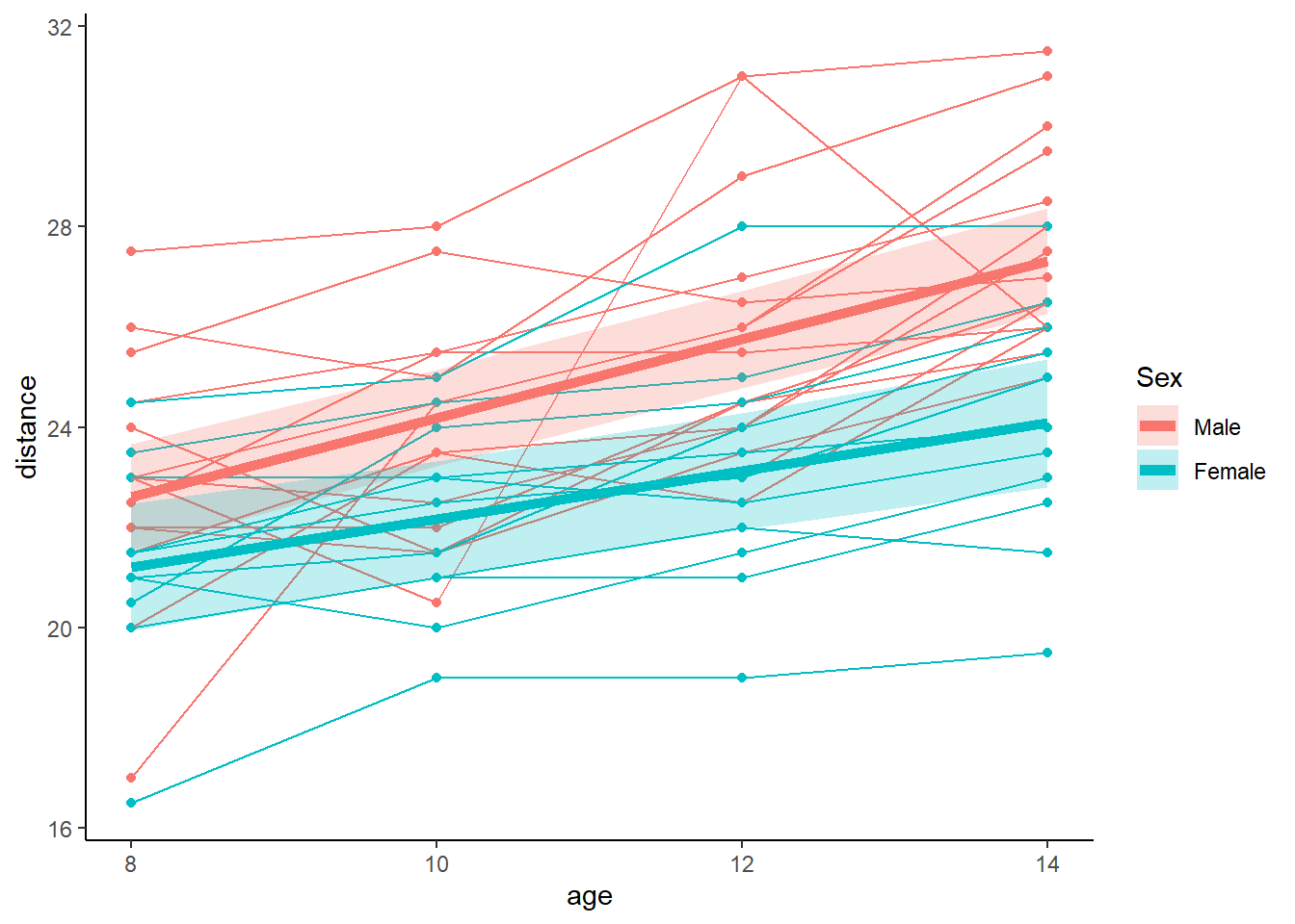 From the plot is each clear that the average trajectory of males is slightly higher than females. The lines run almost parallel, but the males seem to be growing slightly faster.
With the package lmerTest p-values are added to the summary of the model.
library(lmerTest)fm1 <- lmer(distance ~ age*Sex + (1 | Subject), data = Orthodont)
summary(fm1)## Linear mixed model fit by REML. t-tests use Satterthwaite's method [
## lmerModLmerTest]
## Formula: distance ~ age * Sex + (1 | Subject)
## Data: Orthodont
##
## REML criterion at convergence: 433.8
##
## Scaled residuals:
## Min 1Q Median 3Q Max
## -3.5980 -0.4546 0.0158 0.5024 3.6862
##
## Random effects:
## Groups Name Variance Std.Dev.
## Subject (Intercept) 3.299 1.816
## Residual 1.922 1.386
## Number of obs: 108, groups: Subject, 27
##
## Fixed effects:
## Estimate Std. Error df t value Pr(>|t|)
## (Intercept) 16.3406 0.9813 103.9864 16.652 < 2e-16 ***
## age 0.7844 0.0775 79.0000 10.121 6.44e-16 ***
## SexFemale 1.0321 1.5374 103.9864 0.671 0.5035
## age:SexFemale -0.3048 0.1214 79.0000 -2.511 0.0141 *
## ---
## Signif. codes: 0 '***' 0.001 '**' 0.01 '*' 0.05 '.' 0.1 ' ' 1
##
## Correlation of Fixed Effects:
## (Intr) age SexFml
## age -0.869
## SexFemale -0.638 0.555
## age:SexFeml 0.555 -0.638 -0.869At baseline there is no significant difference between males and females. Age is significant, meaning that overall subjects increase with age. The significant interaction denotes the deviation in parallel line seen in the graph.
Test contrasts
The package emmeans can be used to test contrasts and estimate marginal means.
library(emmeans)Examples of use of the package are:
- Compare the difference between male and female at all levels of age
emmeans(fm1, specs = pairwise ~ Sex | age, at = list(age = c(8, 10, 12, 14)))$contrasts## age = 8:
## contrast estimate SE df t.ratio p.value
## Male - Female 1.41 0.844 37.1 1.666 0.1041
##
## age = 10:
## contrast estimate SE df t.ratio p.value
## Male - Female 2.02 0.771 26.3 2.615 0.0146
##
## age = 12:
## contrast estimate SE df t.ratio p.value
## Male - Female 2.63 0.771 26.3 3.406 0.0021
##
## age = 14:
## contrast estimate SE df t.ratio p.value
## Male - Female 3.24 0.844 37.1 3.833 0.0005
##
## Degrees-of-freedom method: kenward-roger- Estimate the marginal means of males and female at age = 10
emmeans(fm1, specs = pairwise ~ Sex | age, at = c(age = 10))$emmeans## age = 10:
## Sex emmean SE df lower.CL upper.CL
## Male 24.2 0.492 26.3 23.2 25.2
## Female 22.2 0.594 26.3 20.9 23.4
##
## Degrees-of-freedom method: kenward-roger
## Confidence level used: 0.95- Compare the overall value at age 12 with age 14:
emmeans(fm1, specs = pairwise ~ age , at = list(age = c(12, 14)))$contrasts## contrast estimate SE df t.ratio p.value
## 12 - 14 -1.26 0.121 79 -10.409 <.0001
##
## Results are averaged over the levels of: Sex
## Degrees-of-freedom method: kenward-roger- Estimate the marginal means at age 8 and 14 for males and females
emmeans(fm1, specs = pairwise ~ age | Sex, at = list(age = c(8, 14)))$emmeans## Sex = Male:
## age emmean SE df lower.CL upper.CL
## 8 22.6 0.539 37.1 21.5 23.7
## 14 27.3 0.539 37.1 26.2 28.4
##
## Sex = Female:
## age emmean SE df lower.CL upper.CL
## 8 21.2 0.650 37.1 19.9 22.5
## 14 24.1 0.650 37.1 22.8 25.4
##
## Degrees-of-freedom method: kenward-roger
## Confidence level used: 0.95